The Starship Engineer's Notebook: Covariance, Contravariance, and the Metric

When we discussed the metric before, in the context of deriving the Lorentz Group, it served to generalize the concept of the dot product into four-dimensions. We've just discussed it in the context of other vector and matrix products as well. Which should be leading naturally to the question of what other function metric tensors might serve. To do so we must introduce a key feature of tensor algebra that has been notably absent thus far, the notion of covariant and contravariant tensors.

Vectors and Duals

Contravariant Vectors

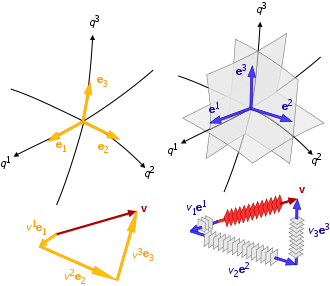
Consider some vector in two dimensional space. The vector itself is a physical or geometric object, it doesn't change no matter how we change its description. We break the vector into two components, along two arbitrarily chosen coordinate axes.

Let's represent the two axes as two unit vectors, one defining x and the other y. We place two vectors pointing along those two directions, creating a basis, which describe the space. Any vector, v can be described by two components which show the projection of v along the basis vectors, e:

$\vec{v}=v^x\vec{e}_x+v^y\vec{e}_y$

If we want to convert to another representation, we would use the Jacobian, the derivative of the new coordinate vectors in terms of the old vectors.

$\vec{v'}=\frac{dv'}{dv}\vec{v}$

To prove this, consider some function f that takes in a scalar value and outputs a vector. Take the derivative of that vector with respect to that scalar in both the original and transformed basis, note that the two derivatives can be related by:

$\begin{align}f\left(\lambda\right)&=\vec{x}\\\frac{\delta\vec{x'}}{\lambda}&=\frac{\delta\vec{x'}}{\delta\vec{x}}\frac{\delta\vec{x}}{\delta\lambda}\end{align}$

For example, let's look at the shift from Cartesian coordinates to polar coordinates:

$\begin{align}r&=\sqrt{x^2+y^2}\\\theta&=\tan^{-1}\left(\frac{y}{x}\right)\\\frac{d{p}'}{d{p}}&=\begin{pmatrix}\frac{dr}{dx}&\frac{dr}{dy}\\\frac{d\theta}{dx}&\frac{d\theta}{y}\end{pmatrix}=\begin{pmatrix}\frac{x}{\sqrt{x^2+y^2}}&\frac{y}{\sqrt{x^2+y^2}}\\\frac{-y}{x^2+y^2}&\frac{x}{x^2+y^2}\end{pmatrix}\\\begin{pmatrix}v^r\\v^\theta\end{pmatrix}&=\begin{pmatrix}v^x\cos\theta+v^y\sin\theta\\\frac{v^y}{r}\cos\theta-\frac{v^x}{r}\sin\theta\end{pmatrix}\end{pmatrix}$

We call objects that transform like this contravariant vectors, usually shortened to just vectors. When we move from one contravariant basis to another contravariant basis, we notice that magnitudes seem to "move" from one component to the other. In a contravariant basis, vector components transform opposite to a change in basis.

Covariant Vectors

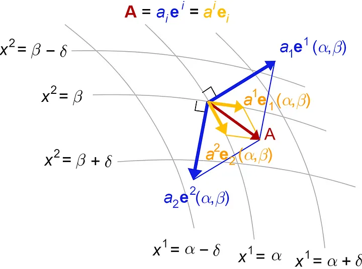
We have another option, however, for representing our coordinate basis. Instead of placing the vectors parallel to the coordinate axes, we can instead have them perpendicular. Rather than lines or curves, we imagine an infinite set of surfaces, where each surface is defined by having the same value for one of its coordinates. This sort of representation is often referred to as one-forms or dual vectors.

Consider some function which takes in a vector and outputs a scalar, each surface of the one-form can be seen as the set of all positions which produce a given value. One-forms can be interpreted as objects which convert vectors to scalars. To see how one-forms transform under a change of basis, consider some function f which takes in a vector and outputs a scalar λ:

$\begin{align}f\left(\vec{x}\right)&=\lambda\\\frac{\delta\lambda}{\delta\vec{x}'}&=\frac{\delta\vec{x}}{\delta\vec{x}'}\frac{\delta\lambda}{\delta\vec{x}}\end{align}$

So we see that one-forms, or covariant vectors, transform opposite from the way contravariant vectors behave. We'll express this relationship, where we will use ~ to represent one-forms:

$\tilde{u}'=\frac{d\tilde{x}}{d\tilde{x}'}\tilde{u}$

and describe the components of a one form using unit one forms:

$\tilde{u}=u_x\tilde{e}^x+u_y\tilde{e}^y$

Relating Vectors And Duals

Let's look at a very simple example of a dual vector. We already know one simple relation that takes in a vector and outputs a scalar, the dot product between two vectors. Writing the dot product as multiplication by a one-form shows:

$\begin{align}\vec{a}\cdot\vec{b}=\tilde{a}\vec{b}&=(a_x\tilde{e^x}+a_y\tilde{e}^y)(b^x\vec{e}_x+b^y\vec{e}_y)=a_x b^x+a_y b^y\\&\rightarrow\left\{\begin{matrix}\tilde{e}^x\vec{e}_x=\tilde{e}^y\vec{e}_y=1\\\tilde{e}^x\vec{e}_y=\tilde{e}^y\vec{e}_x=0\end{matrix}\right.\\&\rightarrow\tilde{e}^i\vec{e}_j=\delta^i_j=\left\{\begin{matrix}1&i=j\\0&i\neq j\end{matrix}\right.\end{align}$

Not only does this give us a relationship between basis vectors and one-forms, it also suggests that there should be a way to convert vectors to one-forms. To find the magnitude of a differential vector dx is another application of the dot product, which will help us find:

$\begin{align}(d\vec{x})^2=(dx)\cdot(dx)&=\sum_{i,j}(dx^i\vec{e}_i)(dx^j\vec{e}j)=\sum_{ij}(dx^i)(dx^j)=\sum_{i}(dx^i)(dx_i)\\&\rightarrow\left\{\begin{matrix}dx_i=\sum_{j}\eta_{ij}dx^j\\\eta_{ij}=\vec{e}_i\cdot\vec{e}_j\end{matrix}\right.\end{align}$

By the same token, if we took the inverse of η we'll see:

$\begin{align}\eta^{-1}&=\eta^{ij}=\tilde{e}^i\cdot\tilde{e}^j\\dx^i&=\sum_{j}\eta^{ij}dx_j\end{align}$

We can see a further property of η by combining these:

$\begin{align}\eta_{ij}\eta^{jk}=(\vec{e}_i\cdot\vec{e}_j)(\tilde{e}^j\cdot\tilde{e}^k)=(\vec{e}_i\tilde{e}^k)(\vec{e}_j\tilde{e}^j)=\delta_i^k\end{align}$

The Metric Tensor

Now that we have found an object that should let us move between contravariant to covariant vectors we should dig deeper into it. Besides performing this one important task, what does it represent? Does it have any geometric meaning?

From Profound Physics

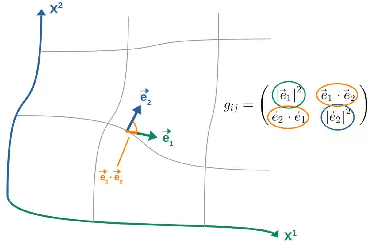
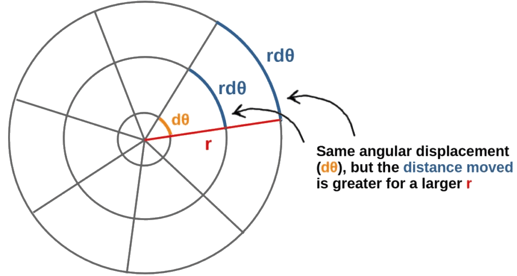
The components of η are dot products of basis vectors, which represent the projection of one basis vector onto one another. For orthogonal coordinate systems, the off-diagonal terms are 0 but for some arbitrary coordinate system there can be non-zero off-diagonal terms. The diagonal terms are the scale factors of the basis vectors. To best understand the scale factors, lets take another look at some vector in polar coordinates:

From Profound Physics

That scale factor is necessary in polar coordinates, so that lengths are properly reflected. The length of some differential element in polar coordinates must include both the radial component and the angular component, both of which must have units of length. The angular component is not just the angle, but a differential arc-length:

$\begin{align}(d\vec{x})^2&=(d\vec{x})\cdot(d\vec{x})=(d\vec{x})^T(\eta)(d\vec{x})=(dr)^2+(r)^2(d\theta)^2\\&=\begin{pmatrix}dr&d\theta\end{pmatrix}\begin{pmatrix}1&0\\0&r^2\\\end{pmatrix}\begin{pmatrix}dr\\d\theta\end{pmatrix}\\\rightarrow\eta_{ij}&=\begin{pmatrix}1&0\\0&r^2\end{pmatrix}\end{align}$

So we know that the metric describes both the geometry of the space and the coordinates being used to describe it. The above example suggests that the metric relates coordinates to distances. For another simple, intuitive example of a curved, two-dimensional space is the surface of a sphere. Just from living on Earth we all know that you can define your location by two angles, latitude and longitude:

To find the distance between any two points, we need the angular separation and also the radius of the sphere. The metric is how we encode the curvature of the space, the radius of the sphere in this case:

$\begin{align}(d\vec{x})^2&=r^2\left((d\theta)^2+(d\phi)^2\sin^2(\theta)\right)\\&=\begin{pmatrix}d\theta&d\phi\end{pmatrix}\begin{pmatrix}r^2&0\\0&r^2\sin^2(\theta)\\\end{pmatrix}\begin{pmatrix}d\theta\\d\phi\end{pmatrix}\end{align}$

Minkowski Metric

Finally, let's head back to discussing flat spacetime. As we discussed before with deriving the Lorentz group, we can find the interval between two events:

$\begin{align}(ds)^2&=-t^2+x^2+y^2+z^2\\&=\begin{pmatrix}t&x&y&z\end{pmatrix}\begin{pmatrix}-1&0&0&0\\0&1&0&0\\0&0&1&0\\0&0&0&1\end{pmatrix}\begin{pmatrix}t\\x\\y\\z\end{pmatrix}\end{align}$

The Minkowski diagram shows the geometry of spacetime. Time moves from the bottom to the top. The origin might be said to represent "here and now." The light lines, ds = 0, oriented at 45º on the image, represent the possible trajectories of light particles. Anything within the light cone (ds < 0) can have a possible causal relationship. We call these time-like curves, because the proper time (dτ = -ds) is positive and time dominates. Curves that venture outside the light cone (ds > 0) are termed spacelike, since the space components dominate. Events that are spacelike separated cannot have any causal link, since such a link would require a faster-than-light signal.

The Minkowski metric above represents flat spacetime. The presence of matter and energy introduces curvature to spacetime. It's also worth noting that the choice of "signature" here is arbitrary. Instead of negative time (dτ = -ds) we could have chosen negative space. The signature can be abbreviated as (- + + +) for negative time and (+ - - -) for negative space.

Einstein Summation Notation

Before moving on, it's important to discuss how we distinguish between covariant and contravariant vectors in notation. For the most part, it's rare to use matrix notation, with → and ~ distinguishing vector from covector, when writing relativistic equations. It's actually most common to simply represent vectors, matrices, and tensors using component indices. I've been following what is the standard notation in discussing relativity, where contravariant terms are superscripted and covariant terms are subscripted:

$\begin{align}\tilde{a}&=a_i\tilde{e}^i\\\vec{b}&=b^i\vec{e}_i\end{align}$

It is assumed in this notation that we sum over all repeated indices. Multiplying by the metric "raises" and "lowers" indices, shifting from contravariant to covariant:

$\begin{align}a_i&=\eta_{ij}a^j\\a^i&=\eta^{ij}a_i\end{align}$

In this notation we express matrices and higher order tensors with more indices, as the metric (a rank-2 tensor) demonstrates above. Performing the same "raising/lowering" operation on some arbitrary rank-3 tensor, T, to demonstrate:

$\eta_{ij}\eta^{kl}T^{im}_k=T^{lm}_j$

We usually call the indices that are being summed over "dummy indices" because they do not appear in the final result. We would also say that we "contract" when the number of indices is reduced, such as when taking the dot product, which is a rank-0 (scalar) quantity constructed from two rank-1 vectors:

$a\cdot b=a^i b_i$

One final bit of notation, it is conventional to represent four-vectors and tensors using Greek letters and purely spatial tensors using Latin letters. For some arbitrary four vector, v, we might write:

$v^\mu=v^0+v^i$

Since we're using index 0 to represent the time component of some four vector, and i represents the space components generally. This notation drastically simplifies the expression of the large, multidimensional tensors of General Relativity.

The Starship Engineer's Notebook

Dropdown Navigation

April 23, 2025

Covariance, Contravariance, and the Metric